Dependent t-Test & Wilcoxon Signed-Rank Test
Prepare
Overview of the Test
A dependent t-test, also called a paired-samples t-test, tests whether there is a difference in outcome scores before versus after participants are exposed to an independent variable.
Because the same participants are measured twice, this is called a within-subjects design.
The normality assumption for a dependent t-test applies to the difference scores, not to the Before and After scores separately.
If the difference scores are normally distributed, use a dependent t-test.
If the difference scores are not normally distributed, use the Wilcoxon Signed-Rank Test.
The dependent t-test is generally preferred when its assumptions are reasonably met because it uses the actual numerical values of the paired observations and can provide greater statistical power for detecting a difference. The Wilcoxon Signed-Rank Test is a useful alternative when the difference scores are not normally distributed.
| Component | Structure | Example |
|---|---|---|
| Research Question | Is there a difference in the outcome scores before versus after the independent variable? | Is there a mean difference in weight (kg) before versus after the exercise program? |
| Null Hypothesis | There is NO difference in the outcome scores before versus after the independent variable. | There is NO difference in weight (kg) before versus after the exercise program. |
| Alternative Hypothesis | There IS a difference in the outcome scores before versus after the independent variable. | There IS a difference in weight (kg) before versus after the exercise program. |
Prepare
RScript Code Template
# install.packages("effsize")
# install.packages("rstatix")

library(readxl)
library(ggpubr)
library(effsize)
library(rstatix)

DatasetName <- read_excel("filepath")

Before <- DatasetName$ScoresBefore
After <- DatasetName$ScoresAfter

Differences <- After - Before

mean(Before, na.rm = TRUE)
median(Before, na.rm = TRUE)
sd(Before, na.rm = TRUE)

mean(After, na.rm = TRUE)
median(After, na.rm = TRUE)
sd(After, na.rm = TRUE)

hist(Differences,
     breaks = 15,
     col = "blue",
     border = "white")

boxplot(Differences,
        main = "Distribution of Score Differences (After - Before)",
        ylab = "Difference in Scores",
        col = "blue",
        border = "darkblue")

# The difference scores boxplot has one outlier.

shapiro.test(Differences)
# The data is normally distributed, (p = .934).

t.test(Before, After, paired = TRUE, na.action = na.omit)

cohen.d(Before, After, paired = TRUE)

# A Dependent T-Test was conducted to determine if there was a difference in weight between Before and After.
# Before scores (M = 7.82, SD = 1.64) were significantly different from After scores (M = 5.21, SD = 1.48), t(19) = 4.12, p < .001.
# The effect size was large, Cohen's d = 0.65.
Step 1
Install & Open the Packages
Packages add additional functionality to R.
| Package | Purpose |
|---|---|
readxl |
Import Excel datasets |
ggpubr |
Create histograms and boxplots |
effsize |
Calculate the effect size for the dependent t-test |
rstatix |
Calculate the effect size for the Wilcoxon Signed-Rank Test |
Install the Packages
Copy-and-paste the following code into your R Script file. Run the installation code once.
install.packages("effsize")
install.packages("rstatix")
You may see warning messages appear when you install a package. These messages do not necessarily mean that the installation failed.
Load the Packages
Copy-and-paste the code below into your R Script. Keep these lines of code in your R Script.
library(readxl)
library(ggpubr)
library(effsize)
library(rstatix)
You must re-open your desired packages every time you start a new RStudio session.
No output will appear. This simply opens the packages so you can use their functions in RStudio.
Step 2
Import & Name the Dataset
Although datasets can be imported entirely through code, many students experience difficulty locating file paths. Therefore, this course uses the point-and-click import method to generate the necessary code automatically.
Import the Excel File
- Select File → Import Dataset → From Excel.
- Select Browse.
- Locate where you saved the downloaded dataset.
- Select the dataset and choose Open.
- Return to the import window and select Import.
What Happens When You Click Import?
Once imported, the dataset will appear in the Environment pane.
RStudio also automatically generates the code used to import the dataset. Copy this line of code into your R Script. This allows the dataset to be automatically imported whenever you reopen your R Script.
General Example
DatasetName <- read_excel("filepath")Example with a Sample File Path
DatasetZ <- read_excel(
"C:/Users/John/OneDrive/Documents/AA5221/Datasets/DatasetZ.xlsx"
)
Step 3
Create Groups for Before & After
Create separate variables for the Before and After scores. Then calculate the difference score for each participant.
This difference score is what we use to check the normality assumption for the dependent t-test.
Code Template
Before <- DatasetName$ScoresBefore
After <- DatasetName$ScoresAfter

Differences <- After - Before
Example
Before <- DatasetName$MedicationA
After <- DatasetName$MedicationB

Differences <- After - Before
Output: None
Step 4
Calculate the Descriptive Statistics
Calculate the mean, standard deviation, and median for the Before and After scores. These descriptive statistics will be used when reporting your results.
Exact Code
mean(Before, na.rm = TRUE)
median(Before, na.rm = TRUE)
sd(Before, na.rm = TRUE)

mean(After, na.rm = TRUE)
median(After, na.rm = TRUE)
sd(After, na.rm = TRUE)
Example Output
[1] 7.82
[1] 7.50
[1] 1.64

[1] 5.21
[1] 5.00
[1] 1.48
Step 5
Normality Check 1: Histogram
Because normality is important, data analysts examine the distribution of the data in several ways before determining which test to use.
For dependent t-tests, we check the normality of the difference scores.
Create the Histogram
For a dependent t-test, the normality assumption applies to the difference scores, not to the Before and After scores separately.
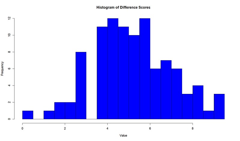
A histogram is a graph that shows how the values of a numerical variable are distributed. It groups values into ranges and uses bars to show how many observations fall within each range.
Exact Code
hist(Differences,
     breaks = 15,
     col = "blue",
     border = "white")
Output: The histogram appears in the Plots pane.
Interpret the Histogram
In your R Script, report whether you think the histogram is normally or abnormally distributed based on a visual assessment.
Specifically, visually determine if you think the histogram has normal skewness (symmetry) and kurtosis (height).
You can calculate statistics such as skewness and kurtosis to describe the shape of a distribution more precisely.
However, we are keeping it simple in this class. You do not need to calculate these statistics by hand.
Instead, use the histogram to visually assess whether the data look approximately normal or noticeably skewed.
In order for data to be considered normal, it must have normal skewness AND kurtosis. Before proceeding, review the Data Visualization and Normality lesson.
Data Visualization and Normality
Reporting Template
# Data for the difference scores appears [abnormally / normally] distributed.
Step 6
Normality Check 2: Boxplot
Before conducting the t-test, create a boxplot to check for potential outliers in the difference scores. An outlier is a score that is unusually high or low compared to the other scores in the dataset. Outliers can affect the distribution of the data and may influence the results of statistical analyses. An outlier can also increase the skewness of a dataset.
Boxplot
A box-and-whisker plot, or boxplot, provides a quick visual summary of a numerical variable. The box shows the middle 50% of the data, the line inside the box shows the median, and the whiskers (lines outside the box) extend to the typical lower and higher values. Individual dots outside the whiskers represent potential outliers. A boxplot allows you to quickly see the center, spread, and unusual values in a continuous variable.

Create the Boxplot
Exact Code
boxplot(Differences,
        main = "Distribution of Score Differences (After - Before)",
        ylab = "Difference in Scores",
        col = "blue",
        border = "darkblue")
Output: The boxplot appears in the Plots pane.
 ```
```
Interpret the Boxplot
In your R Script, report whether the difference scores boxplot has any potential outliers. There are statistical analyses we can use to investigate potential outliers more definitively. However, we will keep things simple for our class.
Look for individual dots beyond the whiskers. Those are potential outliers.
Reporting Template
# The difference scores boxplot does / does not have outliers.
Example
# The difference scores boxplot has one outlier.
What Causes Outliers?
Sometimes the outlier is a legitimate data point. For example, let's say we were collecting data on the average income of a U.S. citizen and, somehow, Elon Musk took our survey. Although his data is legitimate, he would be an outlier that could severely impact our dataset and contribute to a skewed distribution. Sometimes an outlier is due to a survey response error, such as a participant accidentally adding an extra zero to their annual income.
What Do We Do with Outliers?
In more advanced data analytics classes, we investigate potential outliers before deciding what to do with them. Check the original data and consider the value in the context of the variable and research question. Ask: Is this value correct? Does it make sense? Is there a reasonable explanation for why it is unusual? If an outlier is the result of a data-entry or measurement error, it may be appropriate to correct or remove it. If the value is accurate and represents a legitimate observation, do not remove it simply because it is unusual. Any decision to remove an observation should have a clear justification and should be documented. Removing a legitimate outlier can change the distribution, sample size, and results of your analysis.
Step 7
Normality Check 3: Shapiro-Wilk
The Shapiro-Wilk test allows you to check whether the difference scores are normally distributed using a statistical test. The test asks: "Is there a significant difference between my data's distribution and a theoretically perfect normal distribution?"
A p-value greater than .05 indicates that there is not a statistically significant difference between the observed distribution and a normal distribution. A p-value less than .05 indicates that there is a statistically significant difference.
Exact Code
shapiro.test(Differences)Example Output
Shapiro-Wilk normality test

data: Differences
W = 0.99388, p-value = 0.9349
Interpret the Shapiro-Wilk Test
| Shapiro-Wilk P-Value | Meaning | Result |
|---|---|---|
| p > .05 | There is NO significant difference between the data's distribution and a normal distribution. | Data is normal |
| p < .05 | There IS a significant difference between the data's distribution and a normal distribution. | Data is abnormal |
Reporting Template
# Shapiro-Wilk Difference Scores
# The data is [normally / abnormally] distributed, (p = .xxx).
Example
# Shapiro-Wilk Difference Scores
# The data is normally distributed, (p = .934).
Output: The Shapiro-Wilk test results appear in the Console.
Step 8
Select the Correct Test
Was the histogram, boxplot, or Shapiro-Wilk test abnormal? If any of them were abnormal, this would require an investigation.
Since we are keeping our class simple, just look at your Shapiro-Wilk test. Was it normal?
If it was normal, choose the dependent t-test. If it was not normal, choose the Wilcoxon Signed-Rank Test.
Step 9a
Conduct the Dependent t-Test
Conduct the dependent t-test to determine whether there is a statistically significant difference between the Before and After scores.
Exact Code
t.test(Before, After, paired = TRUE, na.action = na.omit)Example Output
Paired t-test

data: Before and After
t = 4.12, df = 19, p-value = 0.0006

alternative hypothesis: true mean difference is not equal to 0

95 percent confidence interval:
0.98 2.87

sample estimates:
mean of the differences
1.92
Step 10a
Calculate Cohen's d (Effect Size)
Exact Code
cohen.d(Before, After, paired = TRUE)Example Output
0.65| Cohen's d | Interpretation |
|---|---|
| ~ 0.20 | Small effect |
| ~ 0.50 | Medium effect |
| ~ 0.80 | Large effect |
| ≥ 1.20 | Very large effect |
Step 11a
Report the Dependent t-Test
After the analyses, report your findings in a few clear sentences in your R Script.
Copy the template and replace the highlighted portions with your output results. There is a standardized method of reporting. DO NOT be creative. Use the provided reporting format.
P-Value Reporting
| p-value | How to Report |
|---|---|
| p < .001 | Report p < .001 |
| .001 < p < .05 | Report the exact p-value to three decimals (example: p = .003) |
| p > .05 | Report p > .05 |
Definitions
- M = mean
- SD = standard deviation
- df = degrees of freedom
- t = t-test value
- p = p-value
For the dependent t-test, degrees of freedom are calculated as the number of paired observations minus 1. For example, if there are 20 participants: df = 20 − 1 = 19.
Report Template
# A Dependent t-Test was conducted to determine if there was a difference in OutcomeVariable between Group1 and Group2.
# Group1 scores (M = xx.xx, SD = xx.xx) were significantly / not significantly different from Group2 scores (M = xx.xx, SD = xx.xx), t(df#) = xx.xx, p = .xxx.
# The effect size was [small / medium / large / very large], Cohen's d = .xxx.
Example Report
# A Dependent t-Test was conducted to determine if there was a difference in weight between Before and After.
# Before scores (M = 7.82, SD = 1.64) were significantly different from After scores (M = 5.21, SD = 1.48), t(19) = 4.12, p < .001.
# The effect size was large, Cohen's d = 0.65.
Step 9b
Conduct the Wilcoxon Signed-Rank Test
Conduct the Wilcoxon Signed-Rank Test to determine whether there is a statistically significant difference between the Before and After scores.
Exact Code
wilcox.test(Before, After, paired = TRUE, na.action = na.omit)Example Output
Wilcoxon signed rank test with continuity correction

data: Before and After
V = 35, p-value = 0.0124

alternative hypothesis:
true location shift is not equal to 0
Step 10b
Calculate the Effect Size
The Wilcoxon effect size is reported as r.
Exact Code
df_long <- data.frame(id = rep(1:length(Before), 2), time = rep(c("Before", "After"), each = length(Before)), score = c(Before, After))
wilcox_effsize(df_long, score ~ time, paired = TRUE)
Example Output
# A tibble: 1 × 4
  .y.    effsize conf.low conf.high
  <chr>    <dbl>     <dbl>      <dbl>
1 score 0.42 0.15 0.66| r Value | Interpretation |
|---|---|
| ~ .10 | Small effect |
| ~ .30 | Medium effect |
| ~ .50 | Large effect |
Step 11b
Report the Wilcoxon Signed-Rank Test
After the analyses, report your findings in a few clear sentences in your R Script.
Copy the template and replace the highlighted portions with your output results. There is a standardized method of reporting. DO NOT be creative. Use the provided reporting format.
P-Value Reporting
| p-value | How to Report |
|---|---|
| p < .001 | Report p < .001 |
| .001 < p < .05 | Report the exact p-value to three decimals (example: p = .003) |
| p > .05 | Report p > .05 |
Definitions
- Mdn = median
- V = Wilcoxon Signed-Rank test value
- p = p-value
Only report the effect size when the results are statistically significant (p < .05).
The Wilcoxon effect size is reported as r.
Report Template
# A Wilcoxon Signed-Rank Test was conducted to determine if there was a difference in OutcomeVariable between Before and After.
# Before scores (Mdn = xx.xx) were [significantly / not significantly] different from After scores (Mdn = xx.xx), V = xx, p = [< .001 / = .xxx / > .05].
# The effect size was [small / medium / large], r = .xxx.
Example Report
# A Wilcoxon Signed-Rank Test was conducted to determine if there was a difference in OutcomeVariable between Before and After.
# Before scores (Mdn = 7.50) were significantly different from After scores (Mdn = 5.00), V = 35, p = .012.
# The effect size was medium, r = .42.
Step 11
Create an RMarkdown File
After completing your R Script, the next step is to convert it into an R Markdown document.
An R Markdown document combines your code, output, and written explanation into a single HTML report. This allows others to reproduce your analysis and view both the code and results in one document.
Before proceeding, review the R Markdown lesson.
Create a New R Markdown File
- Open RStudio.
- Select: File → New File → R Markdown
- Ensure that HTML is selected as the output format.
- Select OK.
You do not need to complete any of the optional fields. The default settings are sufficient for this assignment.
Save the R Markdown File
- Select File → Save As.
- Save the file to your desktop.
- Delete all of the prewritten sample text generated by RStudio.
- Open your completed R Script.
- Copy all of your code.
- Paste the code into the empty R Markdown document.
Create a Code Chunk
R code inside an R Markdown file must be placed inside a code chunk.
Add the following line at the very beginning of your document:
```{r}Then add the following line at the very end of your document:
```All of your code should now be located between the two lines.
Example Structure
```{r}

paste all your code here

```
When the code chunk has been created correctly, the code region will typically appear shaded or highlighted within RStudio.
Step 5: Knit the Document
Once the code chunk has been created, generate the HTML report.
- Select the Knit button at the top of the R Markdown document.
- The Knit button resembles a ball of yarn with a knitting needle.
- Wait for the document to compile.
- A new HTML report should open automatically.
The report will display your code, output, tables, charts, and statistical results in a web-friendly format.
Step 12
Create an RPubs File
After creating and knitting your R Markdown document, the final step is to publish your report to RPubs.
RPubs allows you to share your analysis as a web page that can be viewed in any browser without requiring RStudio.
Before beginning, review the RPubs lesson.
Open Your R Markdown File
- Open your completed R Markdown file.
- Verify that the document knits successfully and displays all output correctly.
- Select the Knit button if you have not already generated the HTML report.
After knitting, the completed HTML report should appear in the Viewer pane or open in a web browser.
Publish to RPubs
- Locate the Publish button in the Viewer pane.
- Select Publish to RPubs.
- Log in to your RPubs account.
- If you do not already have an account, create a free RPubs account.
- Enter a title for your report.
- Optionally enter a description.
- Select Publish.
Save the RPubs HTML File
In addition to publishing the report online, save a copy of the HTML file for your records.
- Open your published RPubs report in a web browser.
- Press Ctrl + S (Windows) or Command + S (Mac).
- Choose a location on your computer.
- If available, select Webpage, HTML Only.
- Save the file.