Independent T-Test & Mann-Whitney U Test
Prepare
Overview of the Test
What Are These Tests?
An Independent T-Test compares the means of two independent groups. For example, you might compare exam scores for females and males.
A Mann-Whitney U Test is the nonparametric alternative used when the outcome variable does not meet the normality assumption required for the independent t-test.
The two groups contain different people or cases. For example, a person belongs to either the Female group or the Male group, but not both.
Tests whether the means of two independent groups are significantly different.
A nonparametric test used to compare two independent groups when the outcome does not meet the normality rule used for the independent t-test.
Prepare
RScript Code Template
Below is an example of what your code will look like. Your code will be different because the dataset name, variable name, expected proportions, results, and interpretations will depend on your assigned dataset.
library(readxl)
library(ggpubr)
library(dplyr)
library(effectsize)
library(effsize)

DatasetName %>%
  group_by(GroupVariable) %>%
  summarise(
    Mean = mean(OutcomeVariable, na.rm = TRUE),
    Median = median(OutcomeVariable, na.rm = TRUE),
    SD = sd(OutcomeVariable, na.rm = TRUE),
    N = n()
  )

hist(DatasetName$OutcomeVariable[DatasetName$GroupVariable == "Group1Name"],
     breaks = 15,
     col = "skyblue",
     border = "white")

hist(DatasetName$OutcomeVariable[DatasetName$GroupVariable == "Group2Name"],
     breaks = 15,
     col = "firebrick",
     border = "white")


ggboxplot(DatasetName,
          x = "GroupVariable",
          y = "OutcomeVariable",
          color = "GroupVariable",
          palette = "jco",
          add = "jitter")


shapiro.test(
  DatasetName$OutcomeVariable[
    DatasetName$GroupVariable == "Group1Name"
  ]
)

shapiro.test(
  DatasetName$OutcomeVariable[
    DatasetName$GroupVariable == "Group2Name"
  ]
)


# Independent t-test


t.test(
  OutcomeVariable ~ GroupVariable,
  data = DatasetName,
  var.equal = TRUE
)

cohens_d_result <- cohens_d(
  OutcomeVariable ~ GroupVariable,
  data = DatasetName,
  pooled_sd = TRUE
)

print(cohens_d_result)


# Mann-Whitney U Test

wilcox.test(
  ExamScores ~ Gender,
  data = DatasetZ
)


# Cliff's Delta

mw_effect <- cliff.delta(
  OutcomeVariable ~ GroupVariable,
  data = DatasetName
)

print(mw_effect)
Step 1
Install & Open the Packages
Install and Load the Packages
You will use several R packages for this analysis.
# Install packages only if you have never installed them before

install.packages("readxl")
install.packages("ggpubr")
install.packages("dplyr")
install.packages("effectsize")
install.packages("effsize")
After the packages are installed, load them with:
library(readxl)
library(ggpubr)
library(dplyr)
library(effectsize)
library(effsize)library() each time you open a new R session.
Step 2
Import & Name the Dataset
Although datasets can be imported entirely through code, many students experience difficulty locating file paths. Therefore, this course uses the point-and-click import method to generate the necessary code automatically.
Import the Excel File
- Select File → Import Dataset → From Excel.
- Select Browse.
- Locate where you saved the downloaded dataset.
- Select the dataset and choose Open.
- Return to the import window and select Import.
What Happens When You Click Import?
Once imported, the dataset will appear in the Environment pane.
RStudio also automatically generates the code used to import the dataset. Copy this line of code into your R Script. This allows the dataset to be automatically imported whenever you reopen your R Script.
General Example
DatasetName <- read_excel("filepath")Example with a Sample File Path
DatasetZ <- read_excel(
"C:/Users/John/OneDrive/Documents/AA5221/Datasets/DatasetZ.xlsx"
)
Step 3
Calculate the Descriptive Statistics
Describe the Two Groups
Start by calculating the mean, median, standard deviation, and sample size for each group.
DatasetZ %>%
  group_by(Gender) %>%
  summarise(
    Mean = mean(ExamScores, na.rm = TRUE),
    Median = median(ExamScores, na.rm = TRUE),
    SD = sd(ExamScores, na.rm = TRUE),
    N = n()
  )
Example Output
# A tibble: 2 × 5
  Gender   Mean Median    SD     N
  <chr>   <dbl>  <dbl> <dbl> <int>
1 Females  83.0   79.3  7.50    50
2 Males    76.7   79.5  6.00    50
Step 4
Normality Check 1: Histogram
Look at the Distribution
Create a histogram for each group. Look for a distribution that is approximately bell-shaped rather than strongly skewed or irregular.
hist(DatasetZ$ExamScores[DatasetZ$Gender == "Females"],
     breaks = 15,
     col = "skyblue",
     border = "white")

hist(DatasetZ$ExamScores[DatasetZ$Gender == "Males"],
     breaks = 15,
     col = "firebrick",
     border = "white")
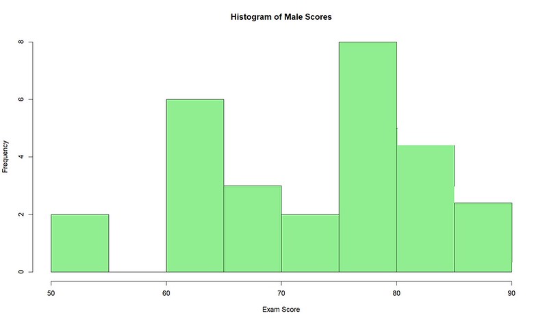
Use the histograms as a visual check. Do not make your final normality decision from the histogram alone.
#Data for Group #1 appears normally / abnormally distributed.
#Data for Group #2 appears normally / abnormally distributed.
Step 5
Normality Check 2: Boxplot
Check for Potential Outliers
A boxplot helps you identify the center, spread, and potential outliers in each group.
ggboxplot(
  DatasetZ,
  x = "Gender",
  y = "ExamScores",
  color = "Gender",
  palette = "jco",
  add = "jitter"
)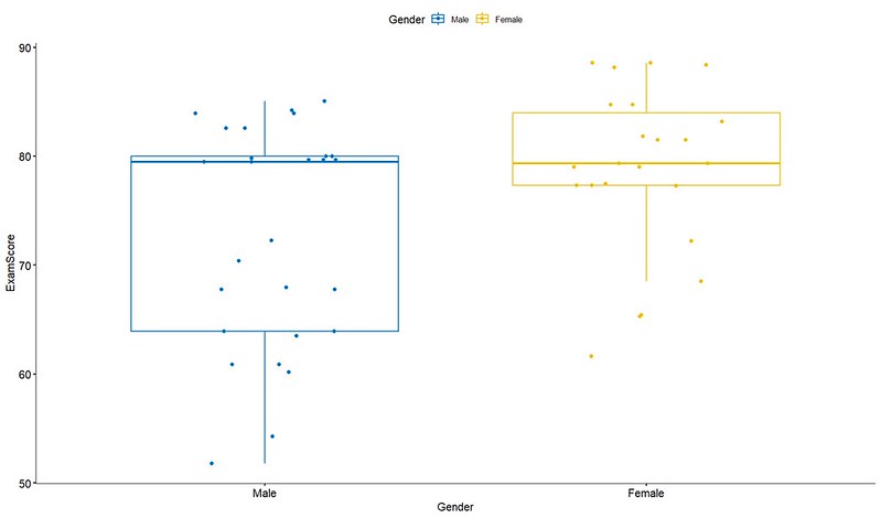
Look for potential outliers in each group. An extreme value can influence the distribution and may contribute to skewness.
For example, if a dataset contains mostly typical incomes but includes one extremely high income, that value could create positive (right) skew.
Step 6
Normality Check 3: Shapiro-Wilk
Conduct the Shapiro-Wilk Test
The Shapiro-Wilk test provides the formal normality check used for this course.
shapiro.test(
  DatasetZ$ExamScores[
    DatasetZ$Gender == "Females"
  ]
)

shapiro.test(
  DatasetZ$ExamScores[
    DatasetZ$Gender == "Males"
  ]
)
Example Output
Females

W = 0.91523, p-value = 0.0778


Males

W = 0.89172, p-value = 0.0611| Shapiro-Wilk p-value | Course Interpretation |
|---|---|
| p > .05 | There is no statistically significant evidence that the distribution differs from a normal distribution. Treat the group as normally distributed for this course. |
| p < .05 | There is statistically significant evidence that the distribution differs from a normal distribution. Treat the group as abnormally distributed for this course. |
#The first group is normally / abnormally distributed (p > or < .05).
#The second group is normally / abnormally distributed (p > or < .05).
Step 7
Select the Correct Test
Choose Your Statistical Test
Use the Shapiro-Wilk results to select the test.
| Normality Results | Test to Use |
|---|---|
| Both groups have p > .05 | Independent T-Test |
| Either group has p < .05 | Mann-Whitney U Test |
Step 9a
Conduct the Independent t-Test
Run the Test
If both groups meet the course normality rule, conduct an Independent T-Test.
For simplicity, this course assumes equal variances and uses var.equal = TRUE.
t.test(
  ExamScores ~ Gender,
  data = DatasetZ,
  var.equal = TRUE
)
Example Output
The following is an abbreviated example. Your output will depend on your dataset.
Two Sample t-test

data:  ExamScores by Gender
t = 4.63, df = 98, p-value < 0.001

sample estimates:
mean in group Females = 83.0
mean in group Males = 76.7Step 9A: Calculate Cohen's d
Calculate the Effect Size
If the Independent T-Test is statistically significant, calculate Cohen's d to determine the size of the difference.
cohens_d_result <- cohens_d(
  ExamScores ~ Gender,
  data = DatasetZ,
  pooled_sd = TRUE
)

print(cohens_d_result)
Example
Cohen's d = 0.93
The exact output from the effectsize package may include additional information, such as a confidence interval. Use the Cohen's d estimate when reporting your effect size.
| Absolute Cohen's d | Course Interpretation |
|---|---|
| 0.00–0.19 | No meaningful difference |
| 0.20–0.49 | Small |
| 0.50–0.79 | Medium |
| 0.80–1.29 | Large |
| 1.30+ | Very large |
Step 10A: Report the Results
Write the Results
Use the following format to report an Independent T-Test.
#An Independent T-Test was conducted to determine if there was a difference
#in OutcomeVariable between Group 1 and Group 2.

#Group 1 scores (M = xx.xx, SD = xx.xx) were significantly different from
#Group 2 scores (M = xx.xx, SD = xx.xx), t(df) = x.xx, p = .xxx.

#The effect size was small/medium/large/very large, Cohen's d = .xx.
Reporting p-values
| Actual p-value | Report as |
|---|---|
| p < .001 | p < .001 |
| .001 ≤ p < .05 | Report the exact p-value to 3 decimal places. |
| p > .05 | p > .05 |
Common Statistical Symbols
| Symbol | Meaning |
|---|---|
| M | Mean |
| SD | Standard deviation |
| df | Degrees of freedom |
| t | Independent T-Test statistic |
| p | Probability value used to determine statistical significance |
For an independent t-test with two groups and equal variances, degrees of freedom are calculated as the total sample size minus the number of groups. For example, with 100 participants and 2 groups: df = 100 − 2 = 98.
Step 8B: Conduct the Mann-Whitney U Test
Run the Test
If either group fails the course normality rule, conduct a Mann-Whitney U Test.
wilcox.test(
  OutcomeVariable ~ GroupVariable,
  data = DatasetName
)
Example
wilcox.test(
  ExamScores ~ Gender,
  data = DatasetZ
)
Example Output
Wilcoxon rank sum test with continuity correction

data:  ExamScores by Gender
W = 30, p-value = 0.002
alternative hypothesis: true location shift is not equal to 0Step 9B: Calculate Cliff's Delta
Calculate the Effect Size
If the Mann-Whitney U Test is statistically significant, calculate Cliff's Delta to determine the size of the group difference.
mw_effect <- cliff.delta(
  OutcomeVariable ~ GroupVariable,
  data = DatasetName
)

print(mw_effect)
Example
Cliff's Delta

delta estimate: 0.45

95 percent confidence interval:
0.21 0.66

Magnitude: medium
The exact output may vary depending on the version of the effsize package and your dataset.
effsize package rather than applying Cohen's d cutoffs to Cliff's Delta.
Step 10B: Report the Results
Write the Results
Use the following format to report a Mann-Whitney U Test.
#A Mann-Whitney U Test was conducted to determine if there was a difference
#in OutcomeVariable between Group 1 and Group 2.

#Group 1 scores (Mdn = xx.xx) were significantly different from
#Group 2 scores (Mdn = xx.xx), W = x.xx, p = .xxx.

#The effect size was small/medium/large, Cliff's Delta = .xx.
Step 11
Create an RMarkdown File
After completing your R Script, the next step is to convert it into an R Markdown document.
An R Markdown document combines your code, output, and written explanation into a single HTML report. This allows others to reproduce your analysis and view both the code and results in one document.
Before proceeding, review the R Markdown lesson.
Create a New R Markdown File
- Open RStudio.
- Select: File → New File → R Markdown
- Ensure that HTML is selected as the output format.
- Select OK.
You do not need to complete any of the optional fields. The default settings are sufficient for this assignment.
Save the R Markdown File
- Select File → Save As.
- Save the file to your desktop.
- Delete all of the prewritten sample text generated by RStudio.
- Open your completed R Script.
- Copy all of your code.
- Paste the code into the empty R Markdown document.
Create a Code Chunk
R code inside an R Markdown file must be placed inside a code chunk.
Add the following line at the very beginning of your document:
```{r}Then add the following line at the very end of your document:
```All of your code should now be located between the two lines.
Example Structure
```{r}

paste all your code here

```
When the code chunk has been created correctly, the code region will typically appear shaded or highlighted within RStudio.
Step 5: Knit the Document
Once the code chunk has been created, generate the HTML report.
- Select the Knit button at the top of the R Markdown document.
- The Knit button resembles a ball of yarn with a knitting needle.
- Wait for the document to compile.
- A new HTML report should open automatically.
The report will display your code, output, tables, charts, and statistical results in a web-friendly format.
Step 12
Create an RPubs File
After creating and knitting your R Markdown document, the final step is to publish your report to RPubs.
RPubs allows you to share your analysis as a web page that can be viewed in any browser without requiring RStudio.
Before beginning, review the RPubs lesson.
Open Your R Markdown File
- Open your completed R Markdown file.
- Verify that the document knits successfully and displays all output correctly.
- Select the Knit button if you have not already generated the HTML report.
After knitting, the completed HTML report should appear in the Viewer pane or open in a web browser.
Publish to RPubs
- Locate the Publish button in the Viewer pane.
- Select Publish to RPubs.
- Log in to your RPubs account.
- If you do not already have an account, create a free RPubs account.
- Enter a title for your report.
- Optionally enter a description.
- Select Publish.
Save the RPubs HTML File
In addition to publishing the report online, save a copy of the HTML file for your records.
- Open your published RPubs report in a web browser.
- Press Ctrl + S (Windows) or Command + S (Mac).
- Choose a location on your computer.
- If available, select Webpage, HTML Only.
- Save the file.